Gradient Boosting Classifier

What’s a Gradient Boosting Classifier?

Gradient boosting classifier is a set of machine learning algorithms that include several weaker models to combine them into a strong big one with highly predictive output. Models of a kind are popular due to their ability to classify datasets effectively.

Gradient boosting classifier usually uses decision trees in model building. But how are the values obtained, processed, and classified?

Classification is a process, where the machine learning algorithm is given some data and puts it into discrete classes. These classes are unique per each data and are categorized accordingly. For example, in our e-mail box we have such categories as “inbox” and “spam”, and the mail received is classified according to the letter’s contextual features.

Regression is also a machine learning algorithm, which works based on the results obtained by the ML model. In the other words, we obtain a real value that is also a continuous value (weight, pulse). Regression aims at predicting value (age of a person) based on continuous values (weight, height, etc.)

Gradient boost was introduced by Jerome Friedman, who believed that with small steps it is possible to predict better with a dataset that is being tested.

To make out predictions and build a decision tree, we will need to carry out several steps.

Step one – Gathering and Analyzing Our Data

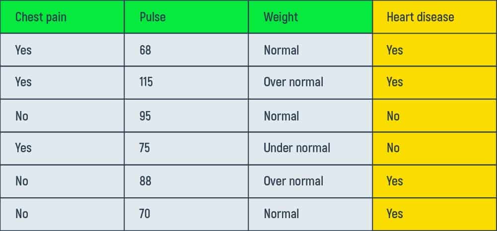
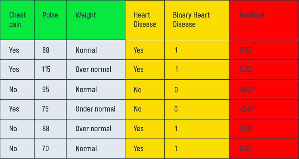
In the table above we are using the training data that we have gathered from six patients. The data shows patients’ presence of chest pain, their pulse (beats per minute), weight (underweight, normal, and overweight), and a history of heart disease. Our aim here is to understand how gradient boost fits a model to this training data.

Step two – Odds and Probability Calculating

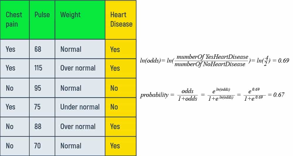
Using gradient boost for classification we discover the initial prediction for every patient in the log (odds).

To calculate the overall log (odds), let’s differentiate between the patients, who answered “yes” for heart disease and the ones, who answered “no”. Here, we have 4 patients in the training dataset that answered positively, and two patients that answered negatively. So, the log (odds) that patients have heart disease is

This number is going to be present in the initial leaf of our tree as an initial prediction.

But how can we use initial prediction for classification? The easiest and smartest way to do so is to convert the log (odds) to probability. The trick here is to use the logistic function.

And our probability will look like this:

With the help of the log (odds) we obtained primarily, the probability of heart disease we get is

The number 0.5 is considered to be the probability threshold in making a classification decision tree based on it, so every number above it makes a patient prone to heart disease automatically. For more information click on the link to watch ROC and AUC machine learning curves.

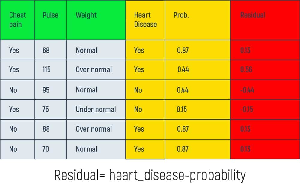
Step three – Residual Calculating

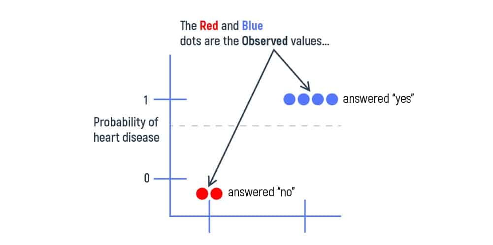
We perform residual calculating to get the difference between the observed and the predicted values. We cannot classify every patient in the training dataset as the one that surely has heart disease because two of these patients did not confirm any heart deviations. So, it is best to measure the initial prediction error with the help of getting the pseudo residual number. Let’s take every “yes” answer as 1 and every “no” answer as 0. Get the idea of why we’re doing this from the graph below:

Here, residual = (binary heart disease – probability) or residual = (yes/no answer – 0.67). We put the obtained results in our table’s new column.

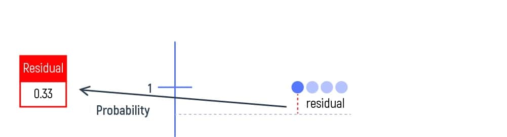
After calculating the residual for each patient, we’ll obtain new values to work within our decision tree’s leaf of initial prediction.

Step four – Building a Decision Tree

To build a decision tree we will need to use the chest pain, pulse, and weight data to predict the tree leaves and residuals. Thus, it is necessary to investigate which column will best describe the obtained results. To do this, we are going to divide our training data into three subtables and build three smaller trees – three weaker models to merge into a strong one later.

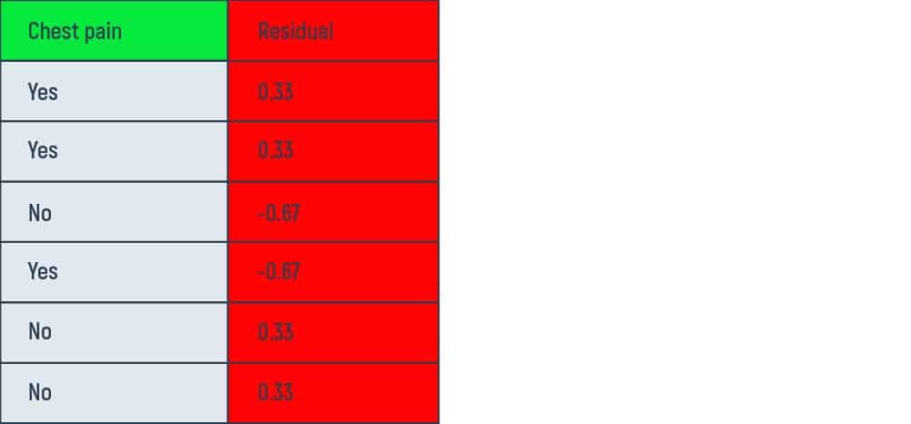
1. Chest pain (binary dataset)

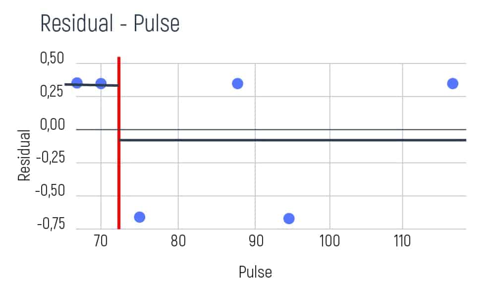
If the answer is “yes” then we will need to find the Residual Sum of Squares (RSS) and the average value of this positive answer.

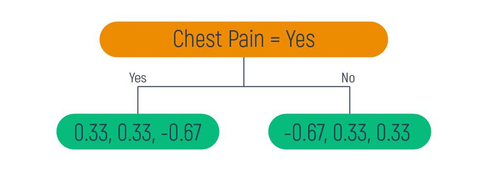
To find the average of the “yes” answer, we should take all the patients, who answered positively, add these numbers and multiply by the quantity of the answers, which is 3. For instance,

Residual sum of Squares or RSS is the sum of the squares of residuals, which indicates errors predicted from actual values of the data set. Small RSS shows that the model perfectly fits the data. Here, average1 and RSS1 are the obtained results, which correspond to the condition of our training model, while average2 and RSS2 are the ones, which do not.

The formula above shows Уi as an element from the residual column. And Ӯ as the average number.

As there is also a “no” answer, we should take it into account and perform the same calculations with regards to the patients, who answered negatively: add the numbers and multiply by 3.

Based on the average value and RSS calculations, we will obtain the following tree leaves:

Here, we have two leaves with residuals but if we want to count the data error, we need to add RSS1 and RSS2 and the result will be the following:

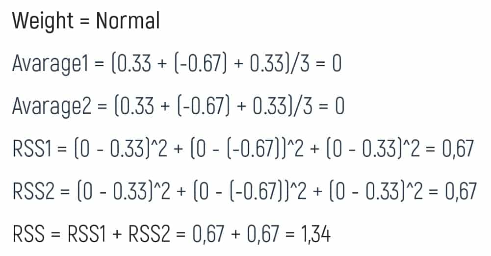
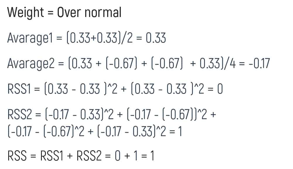
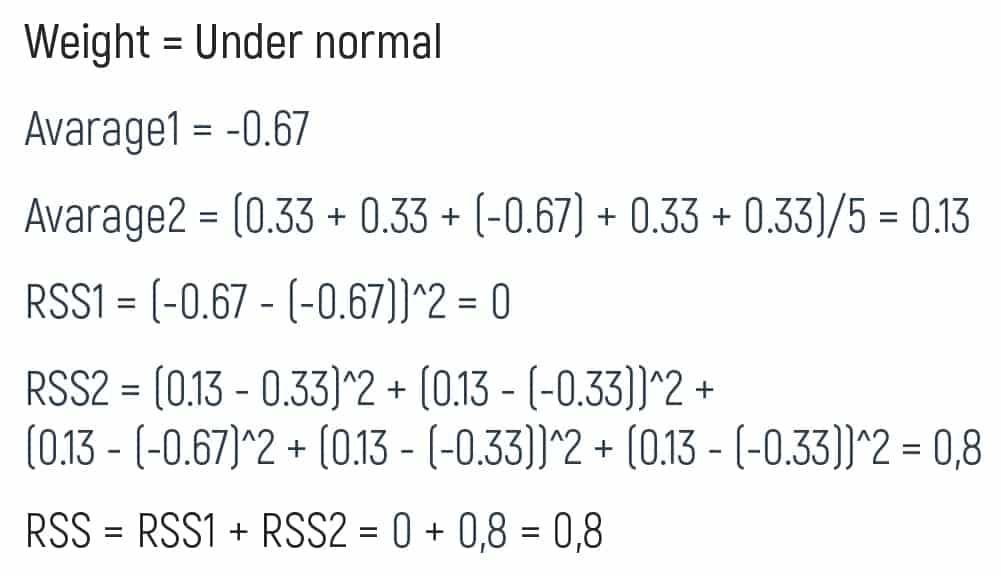
2. Weight (categorical dataset)

To find out the error in the categorical data, it is necessary to divide (or categorize) the weight into such subsections as underweight (lower than normal), normal, and overweight (more than normal).

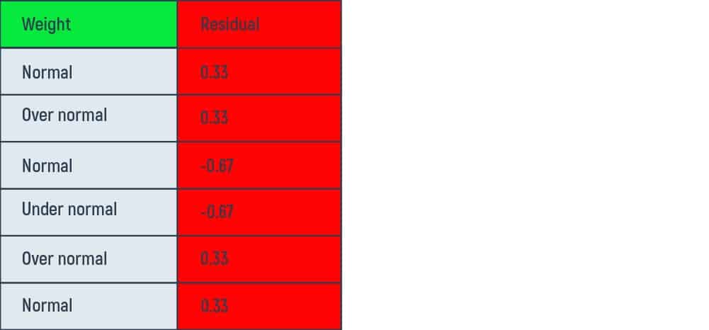
To find residuals and the RSS here, we are following the same steps we carried out before.

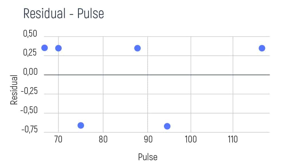
3. Pulse (numerical dataset)

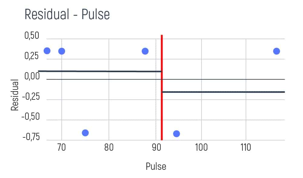
To understand the differences and data errors in pulse, we will need to take several pulse indicators of patients. For example, 68, 70, 75, 88, 95, and 115 beats per minute. Pulse is a numerical value, where the condition is variable. So, we take our pulse values and classify them according to the order of growth. Then, we will need a graph to visualize the variables and the obtained residuals.

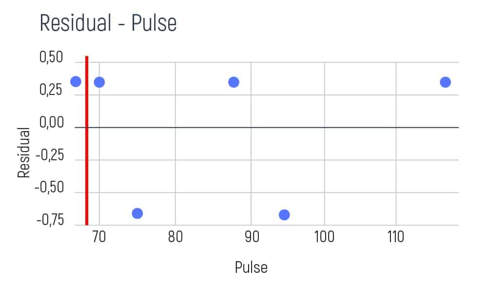
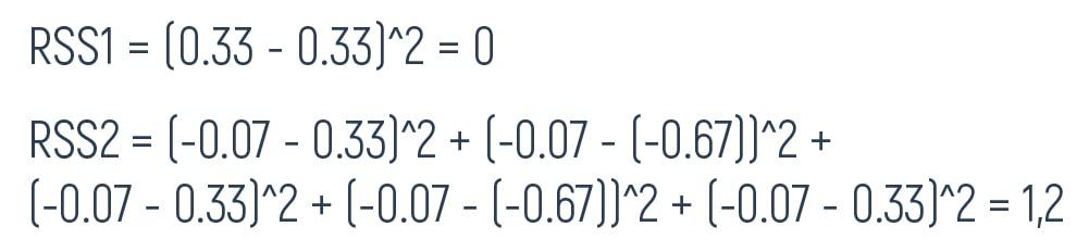
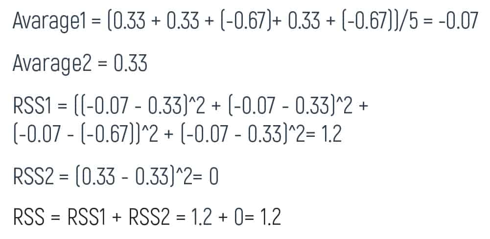
We take the first two values of pulse and calculate their average result. E.g. (68+70)/2=69. Then we show this result as a red line on the graph.

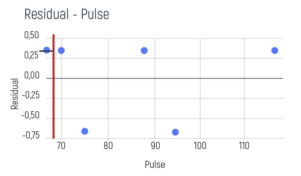
Afterward, we aim to try and find the residual average of the left and the right sides on the graph. As we have only one element on the left, our average is going to be the following:

As the average result is 0.33 we need to show it on our graph. E.g.

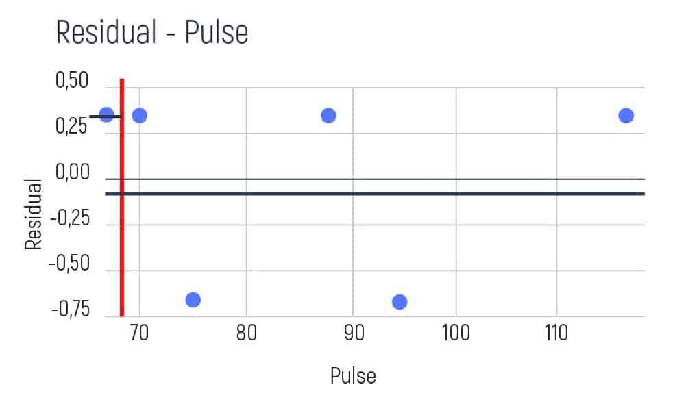
Further, our calculating shifts to the average of the right side of the graph. And it will be:

We’re showing this result on the graph too.

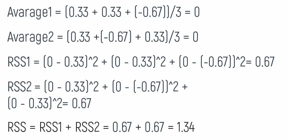
So, the final step is to calculate residuals. This can be done with the help of the following formulas.

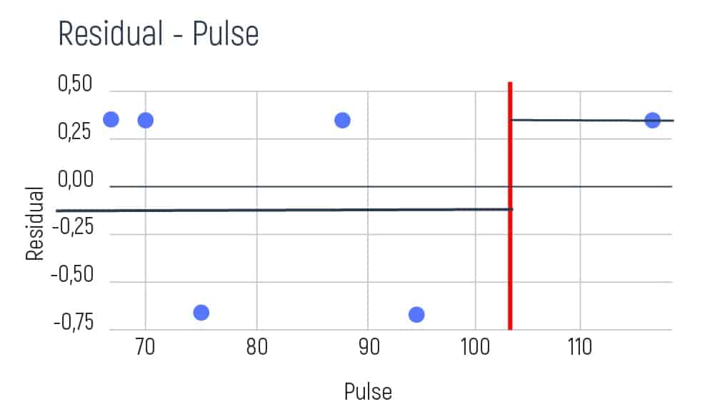
We need to perform the same calculation with all the neighboring values of the pulse. Doing so, we obtain the following results:

Let’s also calculate the same average1/average2, RSS1/RSS2, and the overall RSS value as in the examples above.

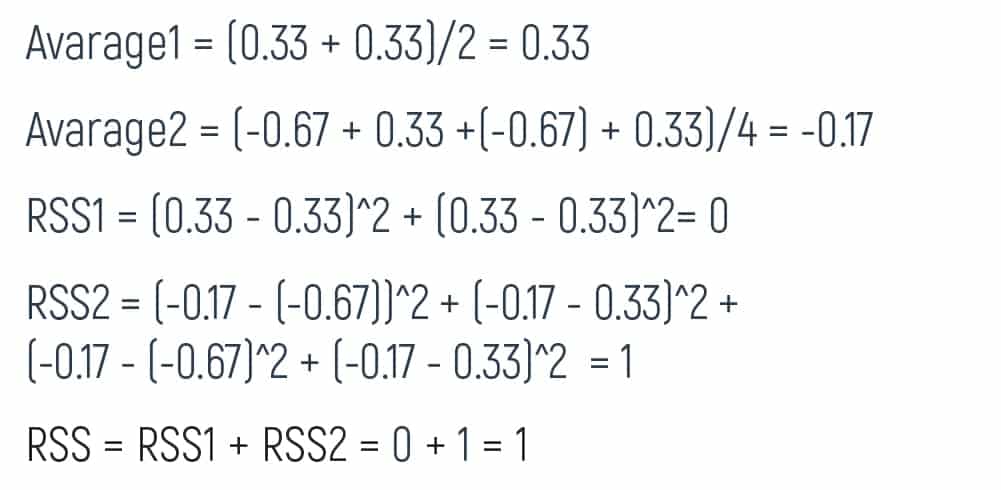
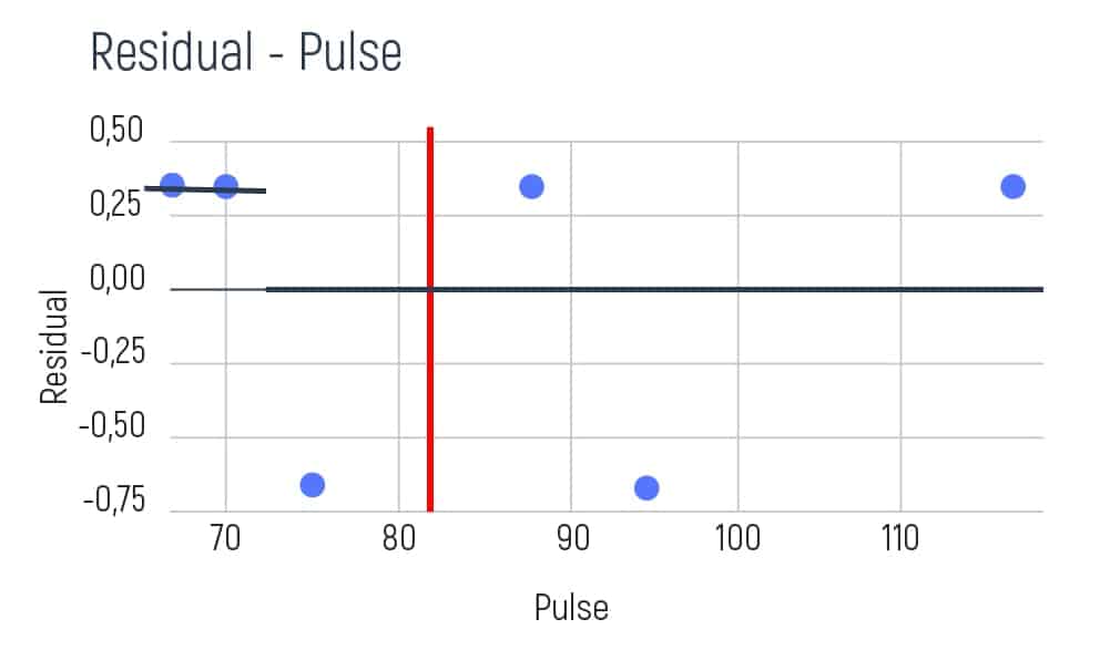
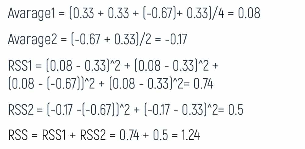
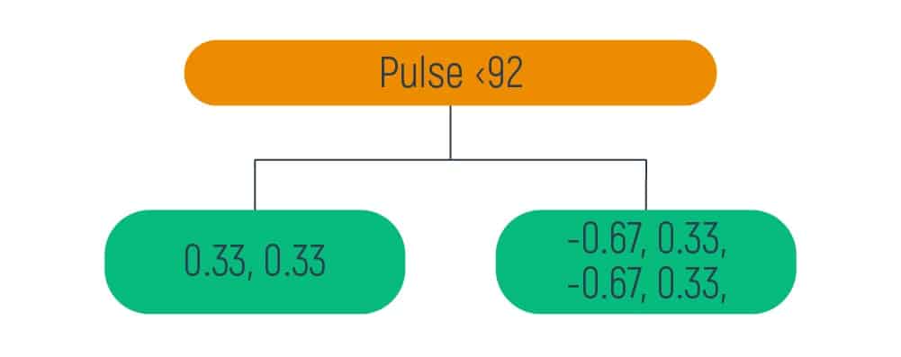
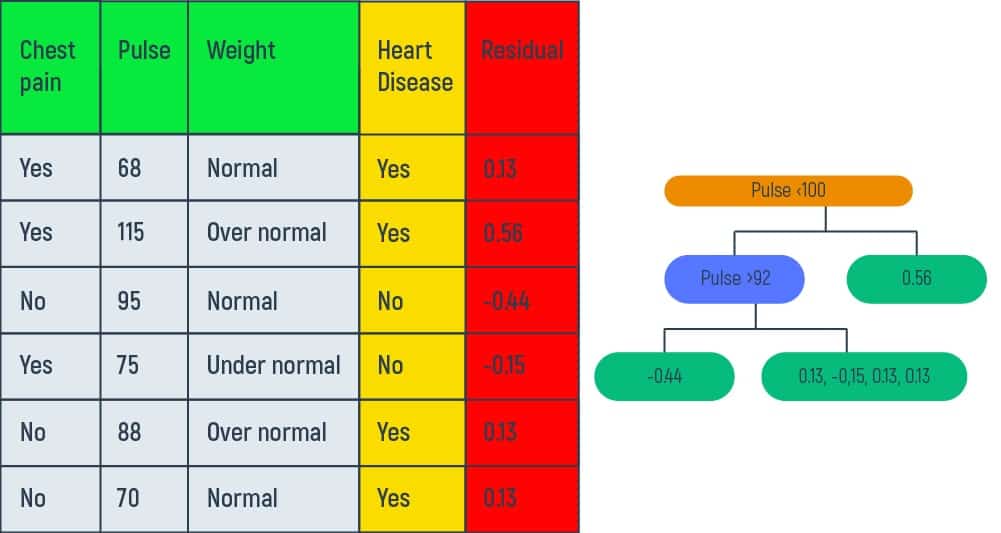
After we obtained all the neighboring results it is necessary to select the best minimal option. This result has been achieved between the pulse range between 70 and 75. Based on this minimal number we can build the following tree:

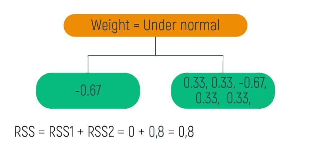
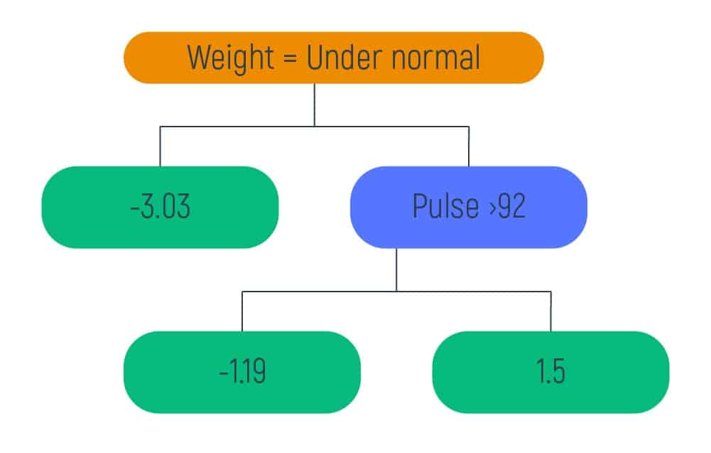
On building a tree with the residuals, the smallest RSS was when we obtained the Weight= Under normal value. So, we take this value as the root of the tree.

Then, it is visually shown that we have only one value on the left leaf and five values on the right leaf. So, we need to carry out the same calculations for the right leaf and obtain a new tree.

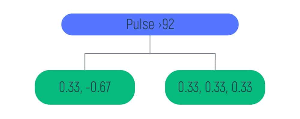
After the calculations are done, we input the obtained data to the right leaf of the previous tree and get the following results:

As we have our data divided into the smallest groups (not more than 3 elements on one leaf) we can move to the next step.

Step 5 – Calculating the Output Value

To calculate the output value we will need to use the following formula:

This formula is the common transformation method, which allows calculating the output value for every leaf.

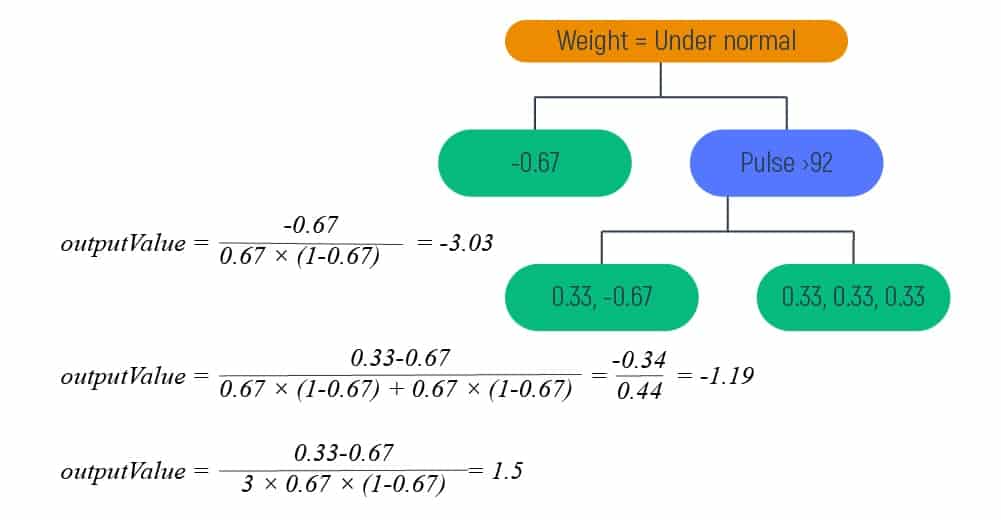
Inputting the already obtained values in the formula we will get the new tree with an output value.

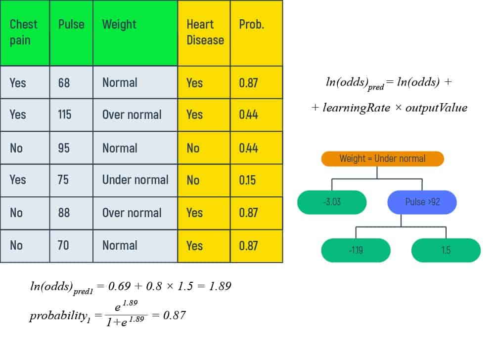
Step Six – Probability Calculating Based on New Values

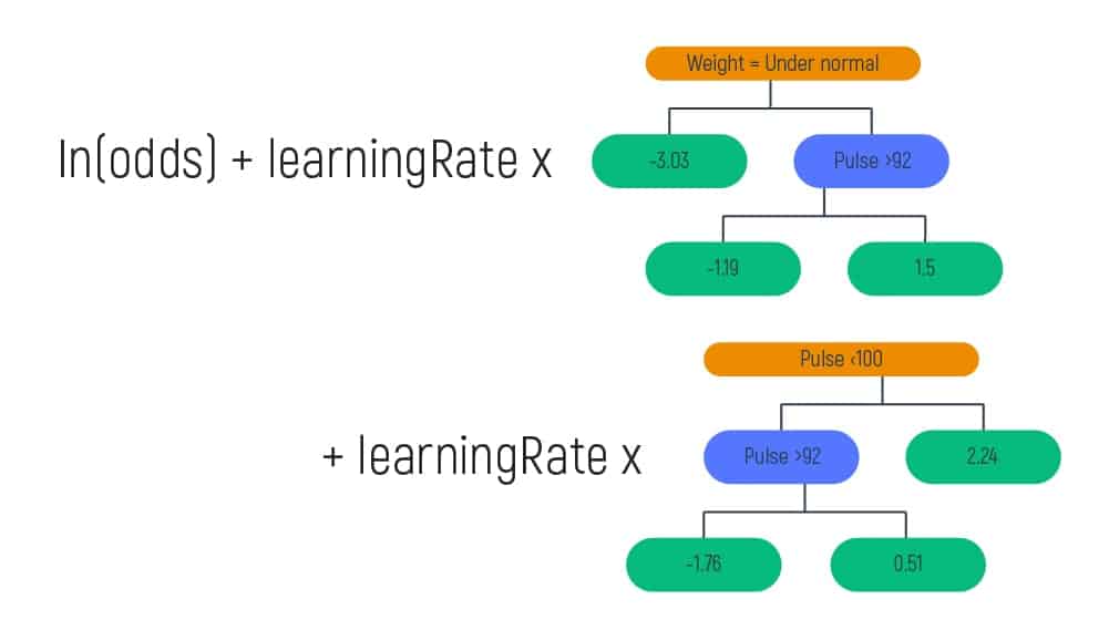
This step requires updating the Predictions section with the new data. So, we are combining the initial leaf with the new tree. And this new tree is scaled by a learning rate, which is 0.8 and it is meant only for illustrative purposes.

This calculation is the same we did before at the beginning of the article. However, the output we get is completely new. And again, after finding out the new probability, let’s find the new residual numbers.

Having the new residuals data it is possible to build a new tree.

The process of tree-building repeats until there is a maximum number of trees specified or the residuals become as small as possible.

To make the example simple, a grading boost has been configured to just two versions of trees. Here, there’s a need to classify a new person as someone who has heart disease or doesn’t have this condition. So, we are doing the same prediction, and calculating the potential probability.

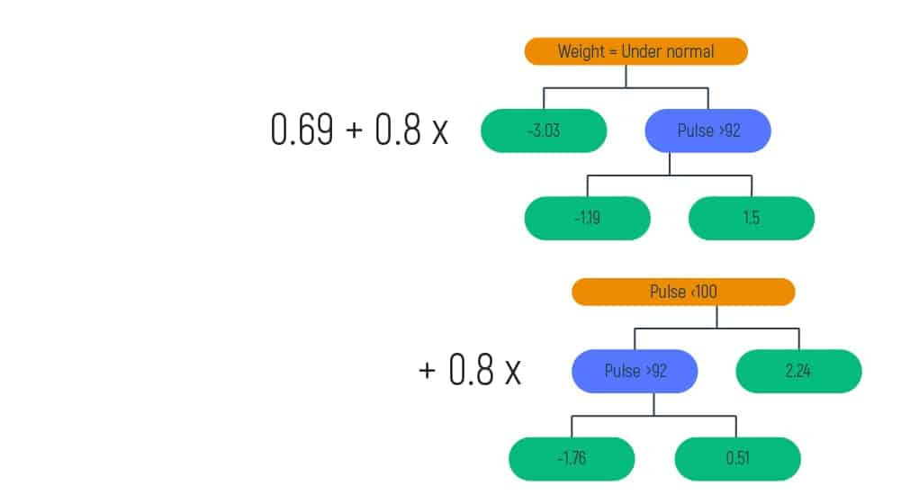
Let’s input into the formula our learning rate, which equals 0.8, and log(odds), which is equal to 0.69. Doing so, we will obtain the following:

But to show you more in detail, imagine we have a new patient and want to calculate the probability of heart disease of this patient.

Let’s calculate our log(odds) predicted with the formula we have:

The result will be:

Using our probability formula we have mentioned in Step 2 we can get our next result.

So, based on the achieved results, our new patient can have heart disease with the probability of 0.95.

Summing Up

The current overview of gradient boosting classifier is shown on a training dataset, but that is the same way it can be used on the real datasets. For instance, if there is a real need to predict whether the patient has a probability of heart disease at present or in the future or not. Thus, now you have an idea of what a gradient boosting classifier is and how it works in classification and tree-building to get accurate predictions and results.

Insights:

1. Understanding Gradient Boosting Classifier: Gradient boosting classifier employs a unique approach by combining multiple weaker models to form a robust predictive model. This technique, introduced by Jerome Friedman, iteratively improves predictions by focusing on the residuals of the previous model. Unlike traditional methods, gradient boosting classifier utilizes small steps to enhance accuracy, making it a powerful tool in machine learning.

2. Data Analysis and Preprocessing: The process of building a gradient boosting classifier begins with thorough data analysis and preprocessing. By examining training data, which typically includes features like chest pain, pulse, and weight, practitioners gain insights into patient characteristics and disease patterns. This step lays the foundation for model training and optimization.

3. Probability Estimation: One of the key aspects of gradient boosting classifier is probability estimation, which involves calculating the likelihood of a patient having a certain condition based on their features. Through odds and probability calculations, practitioners can assign probabilities to different outcomes, enabling informed decision-making in clinical settings.

4. Residual Calculation: Residual calculation is essential for assessing prediction errors and refining the model. By comparing observed and predicted values, practitioners can identify discrepancies and adjust the model accordingly. This iterative process helps improve the model’s accuracy and reliability over time.

5. Tree Building and Optimization: Gradient boosting classifier relies on decision trees to make predictions and classify data. Building decision trees involves dividing the dataset into subsets based on different features, such as chest pain, weight, and pulse. By optimizing tree structures and minimizing prediction errors, practitioners can enhance the model’s predictive capabilities.

6. Output Value Calculation: Calculating the output value is a crucial step in gradient boosting classifier, as it determines the final prediction for each data point. By combining predictions from multiple trees and applying transformation methods, practitioners can generate output values that reflect the likelihood of different outcomes.

7. Iterative Model Improvement: The process of gradient boosting involves iteratively refining the model through successive iterations or “boosting rounds.” By continually updating predictions based on residual errors and adjusting model parameters, practitioners can iteratively improve the model’s performance and predictive accuracy.

8. Probability Estimation for New Data: Once the model is trained and optimized, practitioners can use it to estimate the probability of certain outcomes for new data points. By inputting relevant features into the model and applying probability estimation techniques, practitioners can make informed predictions about patient outcomes and guide clinical decision-making.

9. Clinical Application and Interpretation: Gradient boosting classifier has significant implications for clinical practice, offering healthcare professionals a powerful tool for disease prediction and risk assessment. By leveraging advanced machine learning techniques, practitioners can enhance diagnostic accuracy, improve patient outcomes, and optimize resource allocation in healthcare settings.